“When you can measure what you are speaking about, and express it in numbers, you know something about it.” William Thomson, co-formulator of Thermodynamics
We continually strive to improve the existing OpenSearch features through harnessing the capabilities of OpenSearch itself. One such feature is the Anomaly Detection (AD) plugin, which automatically detects anomalies in your OpenSearch data.
Because OpenSearch is used to index high volumes of data in a distributed fashion, we knew it was essential to design the AD feature to have minimal impact on application workloads. OpenSearch 1.0.1 did not scale beyond 360K entities. Since OpenSearch 1.2.4, it has been possible to track one million entities with a data arrival rate of 10 minutes using 36 data nodes.
While the increase to one million entities was great, most monitoring solutions generate data at a far higher rate. If you want to react quickly to emergent scenarios within your cluster, that 10-minute interval is insufficient. In order for AD to be truly useful, our goal was simple: Shorten the interval to one minute for one million entities, without changing the model output or increasing the number of nodes.
The task of improving AD since its release has mirrored OpenSearch itself—-distributed, dynamic, and not easy to categorize in a linear manner. This post describes the non-linear task of improving AD for all supported OpenSearch versions using the built-in features of OpenSearch. These features include the streamlined access of documents (asynchronous mode, index sorting), changes to system resource management (distributing CPU load, increasing memory), and innovations in the AD model (lower memory, faster throughput).
First steps
At first, it was unclear how to model data characteristics that would measure bottlenecks in a 39-node (36 data nodes, r5.2xlarge Graviton instances) system. Inspired by Thomson, we began testing synthetic periodic functions with injected noise and some anomalies. A rough estimate of model inference time (including time for multiple invocations scoring, supporting explainability features, and updates) was about two-minutes of compute in a 10-minute interval. Clearly, reducing the interval to one-minute would require newer ideas, and we would have to focus on the model.
RCF 2.0 compared with 3.0
One idea was to initiate a Random Cut Forest (RCF) 3.0 model that made scoring and conditional computing of all the explanatory information available through a single API call based on a predictor-corrector architecture reminiscent of a streaming Kalman filter.
RCF was originally designed to flag observations that were too difficult to explain given past data. With RCF 3.0, the algorithm now extends seamlessly to support forecasting and many other capabilities of streaming random forests.
Each model had a dynamic cache internal to the model. Memory consumption corresponded to storing an unused model, whereas the throughput corresponded to a model in use. That difference is germane when each node is processing 1,000,000/36≈27,750 models; the 3x overhead from a fully enlarged model in the running threads would only be dwarfed if we were running 27,750/3≈9,250 threads.
We did not have 9,250 threads. To reduce the number of running threads, we used a dynamic trade-off, switching efficiently between the dynamic and static memory, instead of the static memory-throughput trade-off used from RCF 2.0 used in OpenSearch 1.2.4. When we did, the cache was turned on at the invocation, and all the explanatory computation was performed and discarded afterward.
Since the memory-throughput trade-off was dynamic, we also explored alternate tree representations. In aggregate, we were handling 30 million decision trees. Therefore, any per-tree improvements we could make to size mattered. The newer RCF 3.0 model was at least 2x faster and 30 percent smaller when stored in memory compared to the corresponding usage of RCF 2.0 in OpenSearch 1.2.4.
But this still fell short of our one-minute goal. We would need to change more than the algorithm’s memory throughput and also make tweaks to our CPU usage, especially for OpenSearch 2.0 and above.
CPU usage
In OpenSearch 2.0.1, RCF 3.0 took 30 percent more time when compared with the 2-minute per-interval execution time of OpenSearch 1.2.4. In OpenSearch 1.2.4, the JVM usage was smaller by 30 percent, just as we had expected from smaller models. Also, CPU spikes decreased by 30 percent, even though total execution was larger. To leverage OpenSearch better, we investigated comparable Graviton (r6g.2xlarge) instances and found that CPU spikes were the same as in our baseline (1.2.4) and that the execution time was 20 percent faster. We also looked at using 9 nodes of r6g.8xlarge or r5.8xlarge (both of which have the same vCPUs and RAM in their initial configurations) and found that in both cases, the CPU spikes were 4x smaller.
Still, execution time in OpenSearch 2.0.1 was 1.5x slower than in our baseline. To dig deeper, we looked at the CPU spikes of the original c5.4xlarge nodes in OpenSearch 2.0.1 and found the underlying issue.
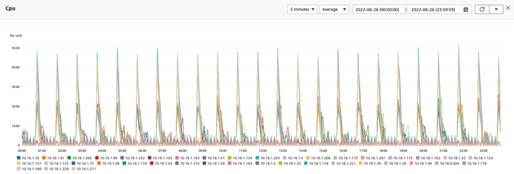
CPU usage stayed around 1 percent, with hourly spikes of up to 65 percent. The spikes were likely caused by the usual culprits: internal hourly maintenance jobs on the cluster, saving hundreds of thousands of model checkpoints and then clearing unused models, and performing bookkeeping for internal states.
For OpenSearch 2.2, we chose to even out the resource usage across a large maintenance window. We also changed the pagination of the coordinating nodes from sync to async mode so that the coordinating nodes did not need to wait for responses before fetching the next page.
Setting up the detector
To set up the detector itself, we used the same category order in our configuration as in our OpenSearch index fields. For example, if the category fields for which we wish to search for anomalies are host and process, and we know that we set indexes to look for the host field before process field, we reflect that order in the category_field:
{
    "name": "detect_gc_time",
    "description": "detect gc processing time anomaly",
    "time_field": "@timestamp",
    "indices": [
        "host-cloudwatch"
    ],
    "category_field": ["host", "process"],
    ...
The detector becomes more efficient when we set it up by using the same field order in our documents and in the sort.field. Therefore, the following example request reflects the same category order: host > process > @timestamp. The body also allocates two nodes for the detector in order to balance shard size.
request_body = {
            "settings":{

              "index": {
                "sort.field": [ "host", "process", "@timestamp"],
                "sort.order": [ "asc", "asc", "desc"],
                "routing.allocation.total_shards_per_node": "2"
              }
           },
           ...
        }
When set up with the same category and sort order, the CPU spikes when using OpenSearch 2.0 were below 25%.
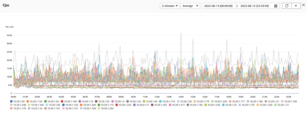
Finally, we achieved continuous anomaly detection of one million entities at a one-minute interval.
Testing for anomalies in the AD plugin
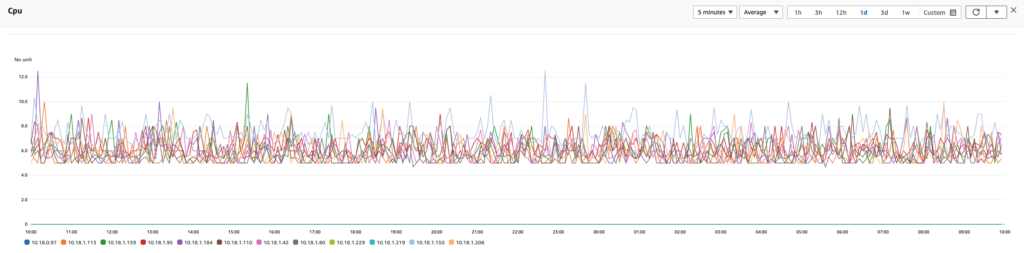
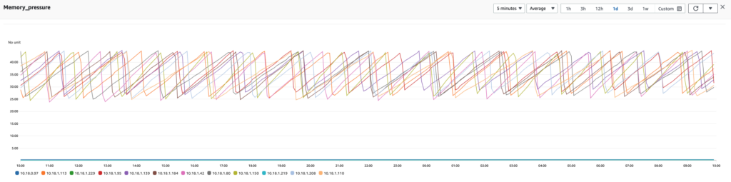
It was serendipitous that the measurements taken from improving the plugin helped us uncover more about the anomalies within the plugin itself. The reading shown in the following image was taken from the plugin’s JVM.
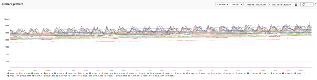
Interestingly, our explorations of the 9 r6g.8xlarge Graviton instances, each with a 128 GB (50 percent) heap, resulted in the measurements seen in the following readings. Notice the lower CPU spikes when compared with our measurements of the same instances from OpenSearch 2.0.
See it for yourself
The improvements outlined in this post are available in OpenSearch 2.2 or greater.
If you want to run this experiment for yourself, remember the following:
- Use the sort.order of the index for which you are detecting anomalies.
- Use the following cluster settings to ensure that 50 percent of dynamic memory is available to the AD plugin, page_size is 10K, and max_entities_per_query is 1 million.
PUT /_cluster/settings
{
    "persistent": {
        "plugins.anomaly_detection.model_max_size_percent": "0.5",
        "plugins.anomaly_detection.page_size": "10000",
        "plugins.anomaly_detection.max_entities_per_query" : "1000000"
    }
}
But what if I don’t use one million entities
From OpenSearch 1.2.4 to OpenSearch 2.2 or greater, many incremental improvements were made to AD, in particular to historical analysis and other downstream log analytics tasks. However, “cold start,” the gap between loading data and seeing results, has been a known challenge in AD since the beginning. Despite this challenge, the cold start gap has decreased from release to release as the AD model has improved.
Because of these improvements over time, the performance of AD is not hampered in more modest cluster settings. To prove this, we performed experiments comparing the recommended testing framework for index/query workloads on a 5-node (2 data node, all c5.4xlarge) cluster both without AD and with AD.
When adding AD, we set AD memory usage to the default 10 percent. We performed each experiment twice (for verification), with two warmup iterations and five test iterations. The final result is the average of these two experiments.
Before each experiment, we restarted the whole cluster, cleared the OpenSearch cache, and removed all existing AD detectors, when applicable.
The following table compares the index latency, CPU and memory usage, GC time and cold start average time with and without AD under the indexing workload.
| Version | query latency P50 (ms) | query latency P90 (ms) | CPU usage P90 (%) | Memory usage P90 (%) | GC time young (ms) | cold start avg (ms) |
|---|---|---|---|---|---|---|
| No AD | ||||||
| 2.3 | 60.958 | 67.33 | 73 | 52.2 | 56,992 | |
| 2.2 | 62.649 | 69.636 | 68 | 52 | 60,831 | |
| 2.1 | 61.693 | 67.782 | 63.333 | 51 | 59,736 | |
| 2.0.1 | 67.682 | 71.785 | 69 | 48 | 59,151 | |
| 1.3.3 | 84.618 | 90.82 | 52 | 44 | 65,240 | |
| 1.2.4 | 77.54 | 85.376 | 61 | 45 | 40,103 | |
| 1.1.0 | 87.33 | 93.147 | 56.625 | 45.5 | 36,206 | |
| 1.0.1 | 77.224 | 82.556 | 62 | 47 | 37,899 | |
| With AD | ||||||
| 2.3 | 97.319 | 106.2 | 68.367 | 53 | 63,722 | 7.93 |
| 2.2 | 106.1 | 114.4 | 69.5 | 52 | 63,293 | 7.85 |
| 2.1 | 108.6 | 117.7 | 66.5 | 47 | 64,242 | 8.4 |
| 2.0.1 | 111.8 | 120.2 | 67 | 53 | 67,764 | 107.81 |
| 1.3.3 | 92.933 | 98.349 | 72 | 42 | 104,510 | 78.87 |
| 1.2.4 | 92.954 | 98.853 | 65.6 | 56 | 67,202 | 132.11 |
| 1.1.0 | 83.545 | 90.319 | 67 | 55 | 61,147 | 985.08 |
| 1.0.1 | 103.6 | 112 | 67 | 48.2 | 39,707 | 600000 |
The following table compares the index latency, CPU and memory usage, GC time and cold start average time with and without AD under the indexing workload.
| Version | index latency P50 (ms) | index latency P90 (ms) | CPU usage P90 (%) | Memory usage P90 (%) | GC time young (ms) | cold start avg (ms) |
|---|---|---|---|---|---|---|
| No AD | ||||||
| 2.3 | 510.6 | 717.8 | 64 | 50 | 13,881 | |
| 2.2 | 510.9 | 709 | 61 | 50 | 13,994 | |
| 2.1 | 515.5 | 723.9 | 77 | 51.333 | 14,227 | |
| 2.0.1 | 534.6 | 755 | 77 | 51.333 | 14,386 | |
| 1.3.3 | 548.6 | 776.4 | 72 | 49 | 30,752 | |
| 1.2.4 | 604.3 | 840 | 64 | 56 | 16,767 | |
| 1.1.0 | 579.3 | 821.6 | 69 | 51 | 16,286 | |
| 1.0.1 | 563.7 | 795.6 | 68.375 | 55 | 16,730 | |
| With AD | ||||||
| 2.3 | 565.5 | 808.5 | 65 | 56 | 17,487 | 9.4361 |
| 2.2 | 530.4 | 731.4 | 63 | 52 | 16,126 | 59.67 |
| 2.1 | 487.2 | 679.7 | 71.5 | 47 | 15,341 | 6.9428 |
| 2.0.1 | 481.3 | 680.5 | 72 | 53 | 21,098 | 71.2371 |
| 1.3.3 | 636.9 | 894 | 85.333 | 45 | 44,675 | 48.7008 |
| 1.2.4 | 618.7 | 870 | 79 | 56 | 30,081 | 47.8312 |
| 1.1 | 622 | 860 | 66.5 | 54.5 | 40,208 | 577.8122 |
| 1.0.1 | 583.4 | 824.7 | 57 | 54.667 | 17,642 | 600000 |
Conclusion
While the benchmark data produced in our experiment could be viewed as less than perfect or perhaps more illustrative of a thought experiment in physics, the improvements were real.
We do expect that explainability, the ability to understand the impact of a model of your nodes, outstrips the demands of inference within analytics. After all, the number of invocations within a model often takes more computational power than accounting for the data running inside. It is simpler to provide explainability based directly on the algorithm being used than to retrofit interpretations. Could streaming algorithms provide a process for invoking multiple API invocations and therefore improve explainability inside the AD model?
If that question or other questions related to machine learning interest you, we would love to hear from you about your experience.
- To discuss topics with other OpenSearch users, start a conversation at forum.opensearch.org.
- To request improvements to the AD plugin, create an issue in the Anomaly Detection plugin repository.