
OpenSearch is widely used for data analytics, especially when working with time-series data. A core feature of time-series analysis is the date histogram aggregation, which groups documents by date or timestamp into defined intervals like months, weeks, or days. This grouping is crucial for visualizing trends and patterns, such as viewing the hourly number of HTTP requests to a website.
However, as data volume grows, the computation required for these aggregations can slow down analysis and dashboard responsiveness. Traditionally, aggregations iterated over every relevant document in order to place it into the correct time bucket, a method that becomes inefficient at scale.
About a year ago, we embarked on an ambitious journey to improve date histogram aggregation performance in OpenSearch. What started as incremental optimizations led to dramatic improvements—in some cases up to 100x faster query responses. This post shares how we achieved those remarkable results and how our optimizations evolved over time.
Why optimize date histograms?: Use cases and benefits
While performance optimizations are valuable in general, they’re especially important for date histograms, which are widely used across various use cases, for example:
- Analyzing web traffic patterns.
- Monitoring application metrics and logs.
- Visualizing sales trends.
- Tracking Internet of Things (IoT) sensor data.
Optimizing date histogram performance offers the following benefits:
- Faster analysis: Reduced dashboard load times for time-series visualizations.
- Improved scalability: Efficient handling of large data volumes without sacrificing performance.
To fully appreciate these optimization opportunities, it’s essential to understand the underlying architecture. The next sections explore the data layout and default execution flow in Lucene and OpenSearch, providing the foundation needed to understand the important optimization details that follow.
How numeric data is stored in OpenSearch
To address performance challenges effectively, OpenSearch introduced optimizations that use the underlying index structure of date fields to significantly accelerate aggregation performance. Before diving into these optimizations, let’s examine how OpenSearch stores numeric data like timestamps using Lucene. Numeric data is stored in two main structures:
- Document values (doc values): A columnar structure optimized for operations like sorting and aggregations. The traditional aggregation algorithm iterates over these values.
- Index tree (BKD tree): A specialized index structure (a one-dimensional BKD tree for date fields) designed for fast range filtering. An index tree consists of inner nodes and leaf nodes. Values are stored only in leaf nodes, while inner nodes store the bounding ranges of their children. This structure allows efficient traversal in a sorted order to find documents within specific ranges.
How aggregation works in OpenSearch
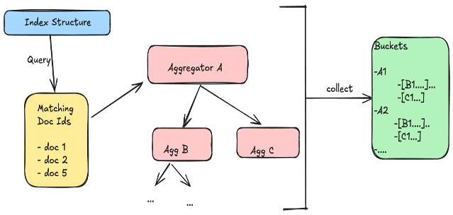
Building on our understanding of data storage, let’s explore how OpenSearch processes aggregations. By default, OpenSearch handles aggregations by first evaluating each query condition on every shard using Lucene, which builds iterators to identify matching document IDs. These iterators are then combined (for example, using logical AND) to find documents that satisfy all query filters. The resulting set of matching document IDs is streamed to the aggregation framework, where each document flows through one or more aggregators. These aggregators use Lucene’s doc values to efficiently retrieve the field values needed for computation (for example, for calculating averages or counts). This streaming model is hierarchical—documents pass through a pipeline of aggregators, allowing them to be grouped into top-level and nested buckets simultaneously. For example, a document can first be bucketed by month, then further aggregated by HTTP status code within that month. This design enables OpenSearch to process complex, multi-level aggregations efficiently in a single pass over the matching documents.
The following diagram illustrates how OpenSearch processes aggregations, from identifying matching documents to collecting results.
Understanding the setup
To validate the aggregation execution model and measure the impact of optimizations in real-world scenarios, we conducted performance testing using the nyc_taxis workload from opensearch-benchmark-workloads. Specifically, we focused on analyzing date histogram aggregation performance using the following query:
{
  "size": 0,
  "query": {
    "range": {
      "dropoff_datetime": {
        "gte": "2015-01-01 00:00:00",
        "lt": "2016-01-01 00:00:00"
      }
    }
  },
  "aggs": {
    "dropoffs_over_time": {
      "date_histogram": {
        "field": "dropoff_datetime",
        "calendar_interval": "month"
      }
    }
  }
}
The query filters documents using a range query on the dropoff time for a 1-year period and computes a date histogram with monthly buckets for the matching documents. The number of nodes in a cluster doesn’t significantly impact the results because the performance bottleneck occurs at the shard level. Thus, we conducted our tests using a single-node cluster. This cluster contained the entire nyc_taxis dataset distributed across a single shard without replicas, allowing us to focus on the core aggregation performance.
Performance bottlenecks
With our test environment in place, we turned our attention to identifying the primary performance bottlenecks. We began by running a single date histogram aggregation query in a loop and collecting flame graphs during the execution, presented in this issue. This analysis revealed two key limitations:
- Data volume dependency: Query latency was directly proportional to data volume. For example, a 1-month aggregation taking 1 second would take 12 seconds for a year’s worth of data.
- Bucket count impact: Using a large number of buckets (for example, minute-level aggregations) caused hash collisions, further degrading performance.
These findings provided crucial insights into the areas requiring optimization, setting the stage for our improvement efforts.
Optimization journey
With a clear understanding of the performance bottlenecks, we embarked on a journey to enhance date histogram aggregation performance. The following sections outline how our optimization efforts evolved over time, from initial enhancements in OpenSearch 2.12 to broader support in OpenSearch 3.0.
Initial attempts
While the identified bottlenecks aligned with our understanding of the aggregation execution flow, we were still surprised by the extent of the performance issues. After all, simply counting the number of documents for each month over a year shouldn’t take 7–8 seconds to return 12 count values! Intrigued by this discrepancy, we initiated some naive optimization attempts, described in the following sections.
Data partitioning
Our first attempt involved splitting the 12-month query into concurrent 6-month operations because the responses from two operations could easily be merged together. While this reduced query time from 8 to 4 seconds (see this comment), community feedback pointed out it was a zero-sum game—we weren’t really reducing CPU usage, just running tasks in parallel. Concurrent segment search already provided these benefits, so this approach offered limited value.
Data slicing
Building on our learnings from the first attempt, we explored a different strategy—data slicing. Instead of using an aggregation query to get the count, we restructured the approach to use a normal range query with track_total_hits enabled to count documents for a single month:
{
  "size": 0,
  "track_total_hits": "true",
  "query": {
    "range": {
      "dropoff_datetime": {
        "gte": "2015-01-01 00:00:00",
        "lt": "2015-02-01 00:00:00"
      }
    }
  }
}
The results were dramatic—query time dropped to about 150 ms for 1 month (see this comment). This meant that even sequential monthly queries completed in about 2 seconds for the whole year, a significant improvement from the original 8 seconds, without increasing concurrency or overall CPU usage.
This remarkable performance difference led us to dive deeper into understanding why this query executed so much faster than the equivalent aggregation query. Our investigation yielded a crucial insight that would shape our next optimization approach.
Phase 1: Filter rewrite
Drawing from our analysis of the range query’s superior performance, we developed the filter rewrite approach. Filter rewrite works by preemptively creating a series of range filters, one for each bucket in the requested date histogram. For example, the monthly aggregation over a year can be rewritten as follows:
{
  "size": 0,
  "aggs": {
    "dropoffs_over_time ": {
      "filters": {
        "1420070400000": {
          "range": {
            "dropoff_datetime": {
              "gte": "2015-01-01 00:00:00",
              "lt": "2015-02-01 00:00:00"
            }
          }
        },
        "1422748800000": {
          "range": {
            "dropoff_datetime": {
              "gte": "2015-02-01 00:00:00",
              "lt": "2015-03-01 00:00:00"
            }
          }
        },
        "1425168000000": {
          "range": {
            "dropoff_datetime": {
              "gte": "2015-03-01 00:00:00",
              "lt": "2015-04-01 00:00:00"
            }
          }
        },
        ...
      }
    }
  }
}
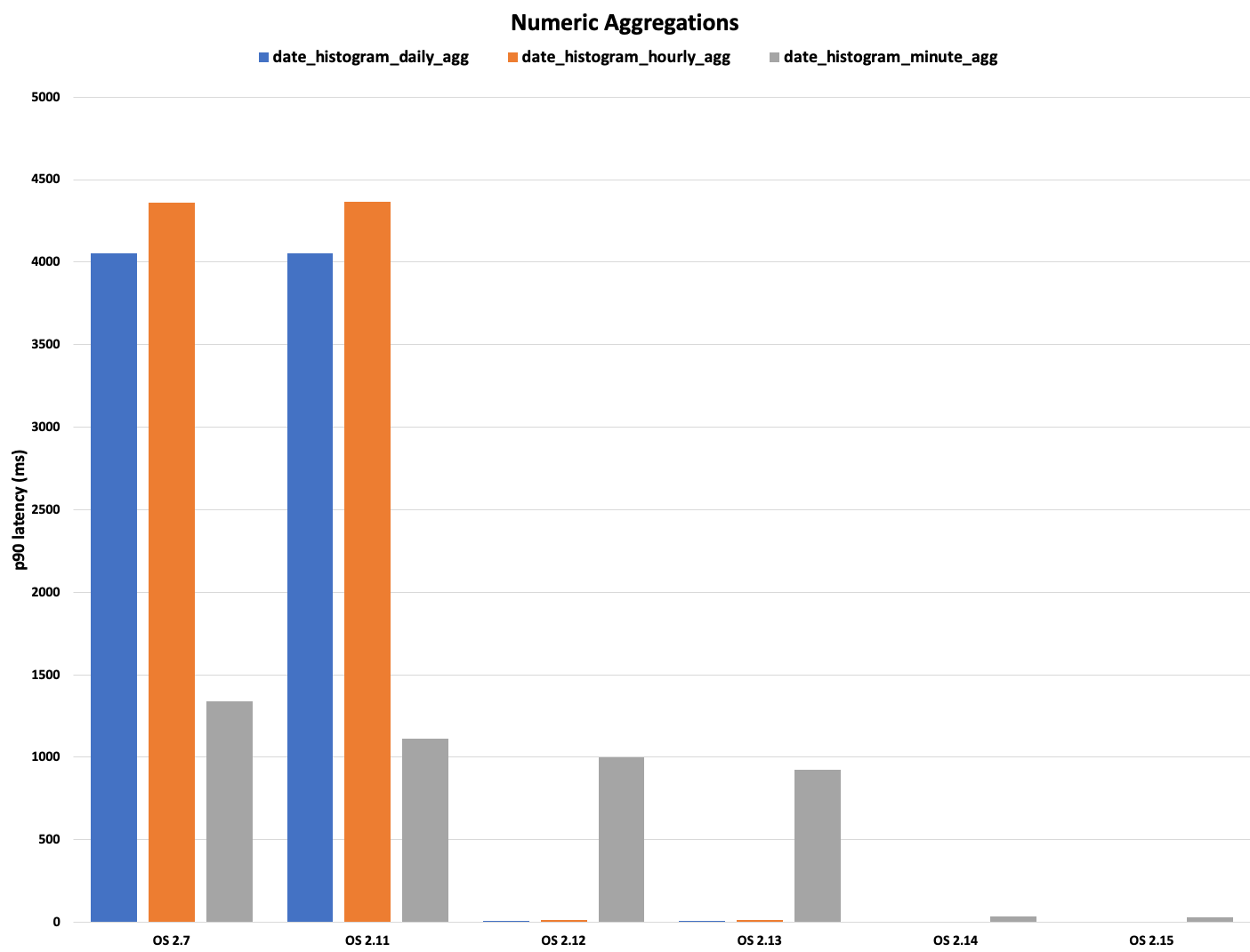
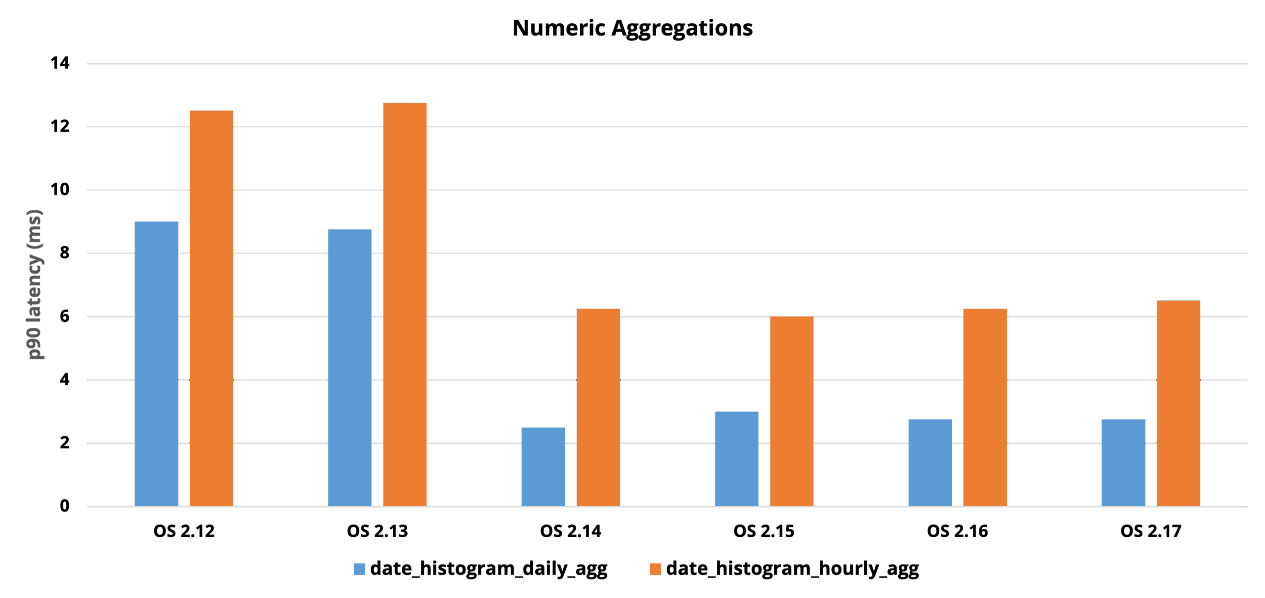
This date histogram aggregation query generates a filter corresponding to each bucket and uses Lucene’s Points Index, which is based on BKD trees, to significantly optimize the aggregation. This tree-based structure organizes data into nodes representing value ranges with associated document counts, enabling efficient traversal. By skipping irrelevant subtrees and using early termination, the system reduces unnecessary disk reads and avoids visiting individual documents. The counts for each bucket are determined using the index tree, similarly to a range query, which is faster than iterating over document values. We also applied this approach to the auto-date histogram, composite aggregation on date histogram source, and, later on, numeric range aggregation with non-overlapping ranges. The following graph shows the performance improvement for daily and hourly date histogram aggregations compared to OpenSearch 2.7 and 2.11. Also notice that the minute-level aggregation (gray bar in the graph) could not initially benefit from this optimization. We discuss this in more detail in the next section.
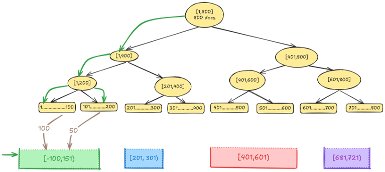
The following diagram illustrates how documents are counted per histogram bucket using the index tree. To efficiently count documents matching a range (for example, 351–771), the traversal begins at the root, checking whether the target range intersects with the node’s range. If it does, the algorithm recursively explores the left and right subtrees.
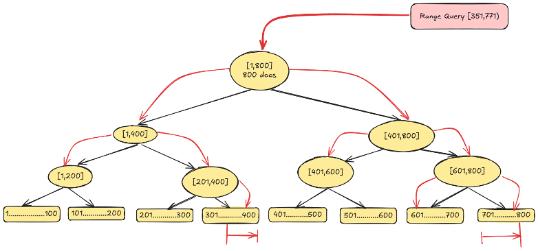
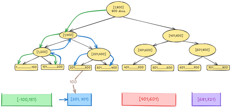
An important optimization involves skipping entire subtrees: if a node’s range falls completely outside the query range (for example, 1–200), it is ignored. Conversely, if a node’s range is fully contained within the query range (for example, 401–600), the algorithm returns the document count from that node directly without traversing its children. This allows the engine to avoid visiting all leaf nodes, focusing only on nodes with partial overlaps. As a result, the operation becomes significantly faster by using the hierarchical structure to skip large irrelevant portions of the tree and aggregate counts efficiently. The optimization workflow is shown in the following diagram.
Phase 2: Addressing scalability using multi-range traversal (OpenSearch 2.14)
The initial tree traversal approach, while effective, had limitations when dealing with a large number of aggregation buckets. Since the algorithm performed a separate tree traversal for each bucket, performance began to degrade as the number of buckets increased. For example, while aggregating monthly log data (12 buckets) showed strong performance improvements, aggregations by minute or hour over long time spans (for example, a year) could involve tens of thousands of buckets. In such cases, the cumulative cost of repeatedly traversing a deep tree from the root for each bucket led to increasing latency and scalability issues (see this issue). This approach was still beneficial for daily or hourly aggregations, in which the number of buckets remained relatively small, yielding up to 50x speed increases in OpenSearch 2.12. However, aggregations by minute remained a bottleneck, prompting the need for a more scalable solution. This led to the development of a new method called multi-range traversal, which aimed to process multiple buckets in a single tree pass, reducing redundant work and greatly improving performance for high-cardinality aggregations.
This approach proved especially effective for minute-level aggregations, where traditional methods struggled to scale. As a result, daily and hourly aggregations saw up to 50x performance improvements, while minute-level aggregations improved by over 100x, with query times dropping from seconds to milliseconds, as shown in the following graph.
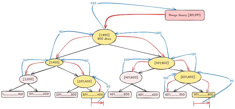
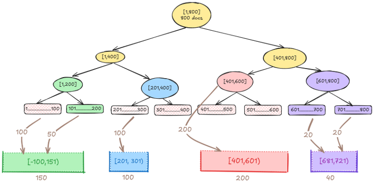
The following diagram illustrates how documents are counted per histogram bucket using multi-range traversal. Instead of restarting the traversal from the top for each bucket, multi-range traversal uses a two-pointer approach: one pointer tracks the current position in the tree, while the other tracks the active bucket.
Because the tree is traversed in sorted order, the algorithm checks whether the current value falls within the range of the active bucket. If it does, the document is collected (see the preceding diagram). If the value exceeds the bucket’s upper bound, the pointer advances to the next bucket (see the following diagram). This seamless transition between buckets avoids restarting the traversal and reduces redundant work. For example, if a node’s range doesn’t overlap with any target bucket (for example, 300–400), it’s entirely skipped.
Similarly, nodes that are fully contained within a bucket (for example, 401–600) are directly counted without further exploration, as shown in the following diagram. This method is especially powerful when dealing with thousands of fine-grained buckets, such as minute-level aggregations, dramatically reducing processing time by minimizing unnecessary operations.
Phase 3: Expanding support for subaggregations (OpenSearch 3.0)
Initially, the optimization only applied to top-level date histograms. However, users frequently need subaggregations within time buckets, such as when calculating average metrics or counting distinct values (for example, average network bandwidth per hour or counts of HTTP status codes). In OpenSearch 3.0, we added support for these subaggregations. Additionally, we implemented protections during development to prevent regressions identified during testing.
Performance results
The optimizations have yielded significant performance improvements:
- Filter rewrite (version 2.12): 10x to 50x improvements observed on specific date histogram queries, compared to the baseline.
- Multi-range traversal (version 2.14): Resolved regressions and achieved further improvements, including up to 70% on the
http_logsworkload and 20–40% onnyc_taxis, compared to the filter rewrite method. - Subaggregation support (version 3.0): 30–40% improvements observed for relevant operations in the
big5workload.
Limitations
While these improvements offer strong performance gains, it’s important to understand when they may not apply or can introduce overhead:
- The filter rewrite optimization primarily applies to
match_allqueries or simplerangequeries compatible with the index tree computation; it does not support arbitrary top-level queries. While segment-levelmatch_allhas been implemented, complex query interactions might still limit filter rewrite applicability. - While multi-range traversal significantly reduced overhead, extremely fine-grained histograms over sparse datasets can potentially still encounter performance regressions.
Conclusion
Index-based optimization for date histogram aggregations in OpenSearch significantly enhances the performance of time-series analysis and visualization. It is applied automatically to eligible aggregations, streamlining your workflows without added manual effort. As OpenSearch evolves, these improvements ensure that you can efficiently gain insights from your data, with less concern about scale.
This journey shows how iterative improvements, deep system understanding, and community collaboration can lead to breakthrough performance gains. While we initially didn’t expect such dramatic results, our commitment to continuous optimization paid off in ways we couldn’t have imagined.
Looking forward
These optimizations have been contributed upstream to Lucene (see this pull request) so that other search systems such as Elasticsearch and Solr can also benefit from these improvements. Looking ahead, we’re continuing to explore and implement further performance enhancements, particularly in the following areas:
- Nested aggregations
- Multi-field queries
- More efficient handling of deleted documents
If you’re interested in collaborating or discussing these topics further, feel free to reach out on GitHub or Slack—we’d love to connect!