With the release of OpenSearch 2.9, we introduced efficient filtering, or “filter-while-search,” functionality for queries using the Facebook AI Similarity Search (Faiss) engine. This update overcomes the previous limitations of pre-filtering and post-filtering in the OpenSearch vector engine. In the OpenSearch 2.10 release, we added support for filtering using the inverted file (IVF) algorithm and further improved the overall performance of efficient filters, allowing users to perform filtered vector similarity search at scale.
Before delving into the intricacies of efficient filters, let’s first grasp the concept of filtering. Filtering empowers users to narrow down their search within a specific subset of their data. In the context of vector search, the objective is to find the nearest neighbor for a query, comprising both the query vector and a filter, among the data points that meet the criteria set by the filter. To illustrate this, let’s explore an example tailored to vector search.
Consider an index in which you are storing a product catalog, where images are represented as vectors. In the same index, you store the ratings, date when it was uploaded, total number of reviews, and so on. The end user wants to search for similar products (providing that as a vector) but wants only products rated 4 or higher. Delivering the desired results for such queries requires filtering along with vector search.
Background
The OpenSearch vector engine includes support for three different engines to perform approximate nearest neighbor (ANN) search: Lucene (Java implementation), Faiss (C++ implementation), and Nmslib (C++ implementation). These engines are simply abstractions of the downstream libraries used for nearest neighbor search. Lucene and Nmslib support the HNSW algorithm for ANN search, while Faiss supports HNSW as well as IVF (with and without product quantization encoding techniques). For more information, you can refer to the k-NN documentation.
As of OpenSearch version 2.8, the vector engine supports three approaches to filtering: scoring script filter (pre-filtering), Boolean filter (post-filtering), and Lucene k-NN filter (which provides efficient filtering functionality but only supports the Lucene engine).
What is efficient filtering?
In vector search, there are basically two types of filtering:
- Pre-filtering means that for a given query that includes one or more filters, you first apply the filters to your complete corpus to produce a filtered set of documents. Then you perform the vector search on those filtered documents. In general, vector search on filtered documents can either be performed through exact search or by creating a new HNSW graph with these filtered document IDs during runtime and then performing the search. These approaches are computationally expensive and scale poorly.
- Post-filtering means that for a given query that includes one or more filters, you first perform the vector search and then apply the filters to the documents that result from the vector search. This approach poses problems because the total number of results can be < k when filters are applied.
As we can see, both pre-filtering and post-filtering have limitations. This is where efficient filtering offers improvements. Let’s first understand the ideas behind efficient filtering for vector search:
- Apply the filters first to identify the filterIds, and while performing the ANN search on the entire corpus, only consider the docIds that are present in the filterIds set.
- Intelligently decide when to perform ANN search on the entire corpus with filterIds and when to perform an exact search. For example, if the filtered document set is small, an ANN search may be less accurate, so efficient filtering should favor accuracy by performing an exact search.
The following diagram shows an example of a vector search flow using efficient filters with Faiss.
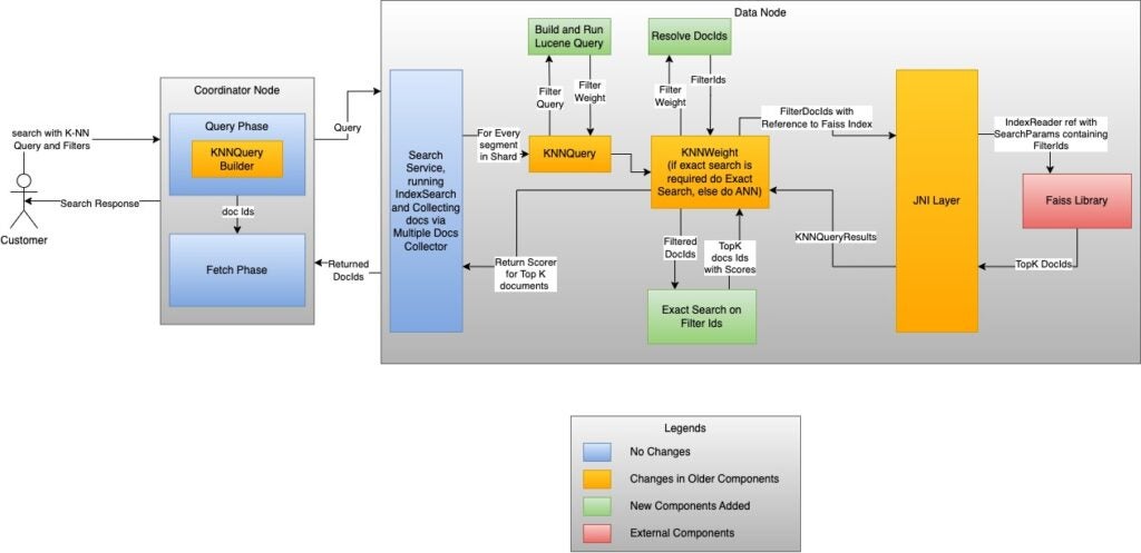
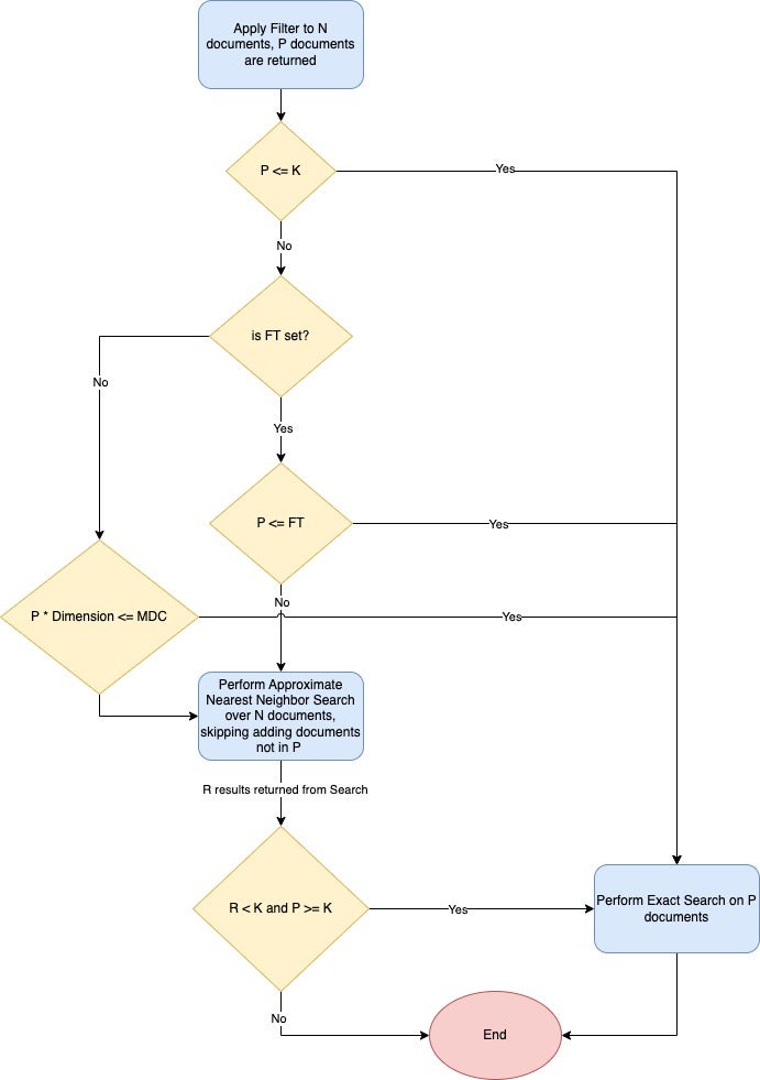
When filtered search is performed on an index using the Faiss engine, the vector search engine decides whether to use ANN filtered search with filters or to perform the exact search. The algorithm uses the following variables:
- N: The number of documents in the index.
- P: The number of documents in the document subset after the filter is applied (P <= N).
- k: The maximum number of vectors to return in the response.
- R: The number of results returned after performing the filtered ANN search.
- FT (filtered threshold): An index-level threshold defined in the
knn.advanced.filtered_exact_search_thresholdsetting that specifies to switch to exact search. - MDC (max distance computations): The maximum number of distance computations allowed in exact search if FT (filtered threshold) is not set. This value cannot be changed.
The following flow chart outlines the algorithm.
Running vector search with efficient filters
First, make sure you have an OpenSearch cluster up and running. Refer to this documentation to set up a full OpenSearch distribution. Before getting into the experiments, let’s go over how to run k-NN workloads in OpenSearch. To get started, you will need to create an index. An index stores a set of documents in such a way that they can be easily searched. For k-NN, the index’s mapping tells OpenSearch what algorithms to use and what parameters to use with them. We’ll start by creating an index that uses HNSW as its search algorithm:
PUT my-hnsw-filter-index
{
	"settings": {
		"index": {
			"knn": true,
			"number_of_shards": 1,
			"number_of_replicas": 0
		}
	},
	"mappings": {
		"properties": {
			"my_vector": {
				"type": "knn_vector",
				"dimension": 4,
				"method": {
					"name": "hnsw",
					"space_type": "l2",
					"engine": "faiss"
				}
			}
		}
	}
}
You can refer to this documentation for more information about different parameters that are supported for index creation.
After the index is created, you can ingest some data:
POST _bulk
{ "index": { "_index": "my-hnsw-filter-index", "_id": "1" } }
{ "my_vector": [1.5, 2.5, 3.5, 4.5], "price": 12.2, "size": "xl" }
{ "index": { "_index": "my-hnsw-filter-index", "_id": "2" } }
{ "my_vector": [2.5, 3.5, 4.5, 5.5], "price": 7.1, "size": "xl" }
{ "index": { "_index": "my-hnsw-filter-index", "_id": "3" } }
{ "my_vector": [3.5, 4.5, 5.5, 6.5], "price": 12.9, "size": "l" }
{ "index": { "_index": "my-hnsw-filter-index", "_id": "4" } }
{ "my_vector": [5.5, 6.5, 7.5, 8.5], "price": 1.2, "size": "l" }
{ "index": { "_index": "my-hnsw-filter-index", "_id": "5" } }
{ "my_vector": [4.5, 5.5, 6.5, 9.5], "price": 3.7, "size": "xl" }
{ "index": { "_index": "my-hnsw-filter-index", "_id": "6" } }
{ "my_vector": [1.5, 5.5, 4.5, 6.4], "price": 10.3, "size": "xl" }
{ "index": { "_index": "my-hnsw-filter-index", "_id": "7" } }
{ "my_vector": [2.5, 3.5, 5.6, 6.7], "price": 5.5, "size": "m" }
{ "index": { "_index": "my-hnsw-filter-index", "_id": "8" } }
{ "my_vector": [4.5, 5.5, 6.7, 3.7], "price": 4.4, "size": "s" }
{ "index": { "_index": "my-hnsw-filter-index", "_id": "9" } }
{ "my_vector": [1.5, 5.5, 4.5, 6.4], "price": 8.9, "size": "xl" }
After adding some documents to the index, you can perform a standard vector similarity search like this:
GET my-hnsw-filter-index/_search
{
	"size": 2,
	"query": {
		"knn": {
			"my_vector": {
				"vector": [ 2, 3, 5, 6],
				"k": 2
			}
		}
	}
}
Now you can use that same index to perform efficient filtering.
Efficient filters
As you can see below, the filter clause is inside the knn query clause. This allows the OpenSearch vector engine to use the docIds produced by the filters to:
- Decide whether to use ANN search or exact search to compute the top K results.
- Guide the ANN search algorithm to choose the right set of DocIds while performing the ANN search using the underlying data structures, like HNSW graphs.
POST my-hnsw-filter-index/_search { "size": 2, "query": { "knn": { "my_vector": { "vector": [2, 3, 5, 6], "k": 2, "filter": { "bool": { "must": [ { "range": { "price": { "gte": 7, "lte": 13 } } }, { "term": { "size": "xl" } } ] } } } } } }
Experiments
Next, run a few experiments to see the tradeoffs and how these different filtering techniques perform in practice. For these experiments, focus on filtered search accuracy and query latency.
Specifically compute the following search metrics:
- Latency p99 (ms), Latency p90 (ms), Latency p50 (ms) – Query latency at various quantiles, in milliseconds
- recall@K – The fraction of the top K ground truth neighbors found in the K results returned by the filtered search
- recall@1 – The fraction of the first ground truth neighbors with the top result returned by the filtered search
The filtering technique will be tested with two types of filters:
- Relaxed filters: In this filter configuration, 80% of the documents are considered for filtered vector search (Filter Spec ref).
- Restrictive filters: In this filter configuration, 20% of the documents are considered for filtered vector search (Filter Spec ref).
From a dataset standpoint, you can use the sift-128 dataset, which has 1 million records of 128 dimensions, and add 3 basic attributes (age, color, taste) with values to all the documents and use them for filtering. You can use this code to achieve that.
To run the experiments, complete the following steps:
- Ingest the dataset into the cluster and run the force merge API to reduce the segment count to 1.
- When ingestion is complete, use the warmup API to prepare the cluster for the search workload.
- Run the 10,000 test queries against the cluster 10 times and collect the aggregated results.
Parameter selection
One tricky aspect of running experiments is selecting the parameters. There are many combinations of parameters to be able to test them all. For example, there are algorithm parameters, like m, ef_search, and ef_construction for HNSW as well as OpenSearch index parameters, like number of shards. That said, you can fix the values of the parameters of the HNSW algorithm for all of the experiments and change the value of number of shards. As with filtering, this variable plays an important role in tuning accuracy and latency. Here are some parameters you can use for these experiments.
| Config Id | m | ef_search | ef_construction | number of shards | K | Size |
|---|---|---|---|---|---|---|
| config1 | 16 | 100 | 256 | 1 | 100 | 100 |
| config2 | 16 | 100 | 256 | 8 | 100 | 100 |
| config3 | 16 | 100 | 256 | 24 | 100 | 100 |
Cluster configuration
| Key | Value |
|---|---|
| Data Node Type | r5.4xlarge |
| Data Node Count | 3 |
| Leader Node | c6.xlarge |
| Leader Node Count | 3 |
The cluster was created using this repo.
Results
Following the process described above, you can expect to achieve the following results.
| Config Id | Filtering Technique | Filter Spec Engine | p50(ms) | p90(ms) | p99(ms) | recall@K | recall@1 |
|---|---|---|---|---|---|---|---|
| config1 | Efficient Filtering Relaxed | Faiss | 17 | 17 | 18 | 0.9978 | 1 |
| config1 | Efficient Filtering Restrictive | Faiss | 27 | 28 | 28 | 1 | 1 |
| Config Id | Filtering Technique | Filter Spec Engine | p50(ms) | p90(ms) | p99(ms) | recall@K | recall@1 |
|---|---|---|---|---|---|---|---|
| config2 | Efficient Filtering Relaxed | Faiss | 11.9 | 12 | 13 | 0.9998 | 1 |
| config2 | Efficient Filtering Restrictive | Faiss | 5 | 6 | 7 | 1 | 1 |
| Config Id | Filtering Technique | Filter Spec Engine | p50(ms) | p90(ms) | p99(ms) | recall@K | recall@1 | |
|---|---|---|---|---|---|---|---|---|
| config3 | Efficient Filtering Relaxed | Faiss | 9 | 9 | 10 | 0.9998 | 1 | |
| config3 | Efficient Filtering Restrictive | Faiss | 4 | 5 | 8 | 1 | 1 |
Conclusion
In this post, we covered how efficient filters work with vector search in OpenSearch. As you can see in the results, you can run experiments that demonstrate 0.99 recall@K and 1 recall@1 across all shard configurations for a similar dataset. The latencies in the experiments change with the change in number of shards, which is expected because you will achieve greater parallelism with a higher number of shards.
FAQs
What filters are best for my use case?
Please refer to this table for information regarding what filters should be used in a given scenario. We continue to update this table as new filter optimizations are introduced.
What engines can I use efficient filters for?
Efficient filters are supported in the Faiss engine with the HNSW algorithm (k-NN plugin versions 2.9 and later) or the IVF algorithm (k-NN plugin versions 2.10 and later). Before OpenSearch 2.9, efficient filters were only supported in the Lucene engine and were called Lucene Filters. Please refer to this documentation for the latest support matrix.
References
- Meta issue: https://github.com/opensearch-project/k-NN/issues/903
- Filters enhancement for restrictive filters: https://github.com/opensearch-project/k-NN/issues/1049