


A practical guide to selecting HNSW hyperparameters
Vector search plays a crucial role in many machine learning (ML) and data science pipelines. In the context of large language models (LLMs), vector search powers retrieval-augmented generation (RAG), a technique that retrieves relevant content from a large document collection to improve LLM responses. Because finding exact k-nearest neighbors (k-NN) is computationally expensive for large datasets, approximate nearest neighbor (ANN) search methods, such as Hierarchical Navigable Small Worlds (HNSW), are often used to improve efficiency [1].
Optimizing HNSW: Balancing search quality and speed
Configuring HNSW effectively is a multi-objective problem. This blog post focuses on two key objectives:
- Search quality, measured by recall@k—the fraction of the top k ground truth neighbors that appear in the k results returned by HNSW.
- Search speed, measured by query throughput—the number of queries executed per second.
While index build time and index size are also important, we will leave those aspects for future discussion.
The structure of the HNSW graph is controlled by its hyperparameters, which determine how densely vectors are connected. A denser graph generally improves recall but reduces query throughput, while a sparser graph has the opposite effect. Finding the right balance requires testing multiple configurations, yet there is limited guidance on how to do this efficiently.
Key HNSW hyperparameters
The three most important hyperparameters in HNSW are:
M– The maximum number of graph edges per vector. Higher values increase memory usage but may improve search quality.efSearch– The size of the candidate queue during search. Larger values may improve search quality but increase search latency.efConstruction– Similar toefSearchbut used during index construction. Higher values improve search quality but increase index build time.
Finding effective configurations
One approach to tuning these hyperparameters is hyperparameter optimization (HPO), an automated technique that searches for the optimal configuration of a black-box function [5, 6]. However, HPO can be computationally expensive while providing limited benefits [3], especially in cases where the underlying algorithm is well understood.
An alternative is transfer learning, where knowledge gained from optimizing one dataset is applied to another. This approach helps identify configurations that approximate optimal results while maintaining efficiency [3, 4].
Recommended HNSW configurations
In the next section, we introduce a method for selecting HNSW configurations. Based on this approach, we provide five precomputed configurations that progressively increase graph density. These configurations cover a range of trade-offs between search quality and speed across different datasets.
To optimize your search performance, you can evaluate these five configurations sequentially, stopping once recall meets your requirements. Because the configurations are ordered by increasing search quality, testing them in this order is likely to yield better search quality with each step:
{'M': 16,  'efConstruction': 128, 'efSearch': 32}
{'M': 32,  'efConstruction': 128, 'efSearch': 32}
{'M': 16,  'efConstruction': 128, 'efSearch': 128}
{'M': 64,  'efConstruction': 128, 'efSearch': 128}
{'M': 128, 'efConstruction': 256, 'efSearch': 256}
Portfolio learning for HNSW
Portfolio learning [2, 3, 4] selects a set of complementary configurations so that at least one performs well on average when evaluated across different scenarios. Applying this approach to HNSW, we aimed to identify a set of configurations that balance recall and query throughput.
To achieve this, we used 15 vector search datasets spanning various modalities, embedding models, and distance functions, presented in the following table. For each dataset, we established ground truth by computing the top 10 nearest neighbors for every query in the test set using exact k-NN search.
| Dataset | Dimensions | Train size | Test size | Neighbors | Distance | Embedding | Domain |
|---|---|---|---|---|---|---|---|
| Fashion-MNIST | 784 | 60,000 | 10,000 | 100 | Euclidean | - | Image, cloth |
| MNIST | 784 | 60,000 | 10,000 | 100 | Euclidean | - | Image, digits |
| GloVe | 25 | 1,183,514 | 10,000 | 100 | Angular | Word-word co-occurrence matrix | Language (wiki, common crawl) |
| GloVe | 50 | 1,183,514 | 10,000 | 100 | Angular | Word-word co-occurrence matrix | Language (wiki, common crawl) |
| GloVe | 100 | 1,183,514 | 10,000 | 100 | Angular | Word-word co-occurrence matrix | Language (wiki, common crawl) |
| GloVe | 200 | 1,183,514 | 10,000 | 100 | Angular | Word-word co-occurrence matrix | Language (wiki, common crawl) |
| NY Times | 256 | 290,000 | 10,000 | 100 | Angular | BoW | Language, news article |
| NY Times | 16 | 290,000 | 10,000 | 100 | Angular | BoW | Language, news article |
| SIFT | 128 | 1,000,000 | 10,000 | 100 | Euclidean | SIFT descriptors | Image |
| SIFT | 256 | 1,000,000 | 10,000 | 100 | Hamming | SIFT descriptors | Image |
| Last.fm | 65 | 292,385 | 50,000 | 100 | Inner product | Matrix factorization | Song recommendation |
| Word2bits | 800 | 399,000 | 1,000 | 100 | Hamming | Word2Vec with quantized parameter | Language, English Wikipedia |
| GIST | 960 | 1,000,000 | 1,000 | 100 | Euclidean | GIST descriptors, INRIA C implementation | Image |
| MS MARCO | 384 | 1,000,000 | 50,000 | 100 | Euclidean | MiniLLM | Language, Question answering |
| openai-dbpedia | 1,536 | 950,000 | 50,000 | 100 | Euclidean | text-embedding-3-large | Language, DBPedia |
For each dataset, we evaluated a grid of 80 HNSW configurations based on the following search space:
search_space = {
    "M": [8, 16, 32, 64, 128],
    "efConstruction": [32, 64, 128, 256],
    "efSearch": [32, 64, 128, 256]
}
For these experiments, we used an OpenSearch 2.15 cluster with three cluster manager nodes and six data nodes, each running on an r6g.4xlarge.search instance. We evaluated test vectors in batches of 100 and recorded query throughput and recall@10 for each HNSW configuration. In the next section, we introduce the algorithm used to learn the portfolio.
Method
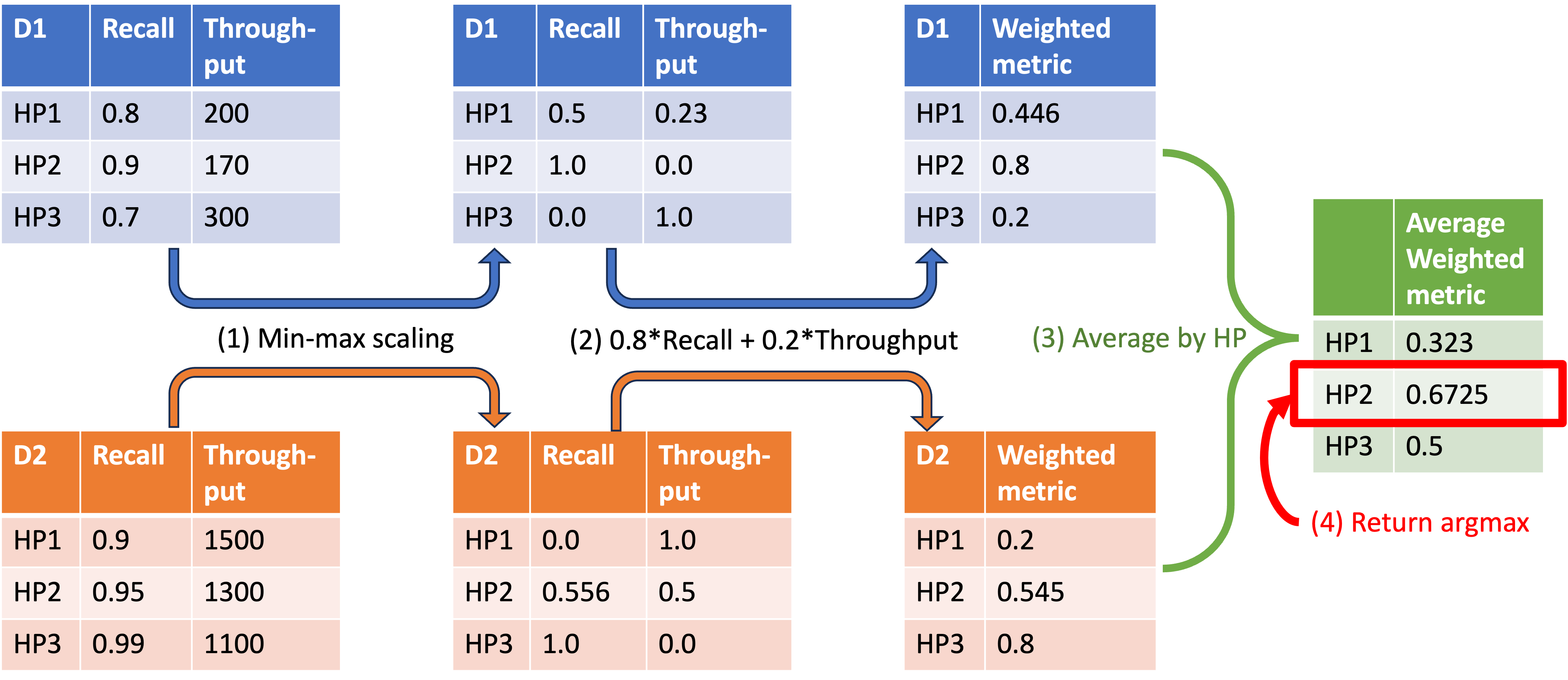
To capture different trade-offs between recall and throughput, we used a simple linearization approach, assigning values between 0 and 1, inclusive, to both recall and throughput. Given a specific weighting, we identified the configuration that maximizes the linearized object using the following four steps:
- Normalize recall and throughput – Apply min-max scaling within each dataset so that recall and throughput values are comparable.
- Compute weighted metric – Using the assigned weights, combine the normalized recall and throughput into a new weighted metric.
- Average across datasets – Calculate the average weighted metric across datasets.
- Select the best configuration – Identify the configuration that maximizes the average weighted metric.
The following figure illustrates the algorithm using an example with two datasets and three configurations.
We used the following weighting profiles for recall and throughput. We did not assign higher weights to throughput because most applications prioritize achieving good recall before optimizing for throughput.
| 0 | 1 | 2 | 3 | 4 | |
|---|---|---|---|---|---|
w_recall |
0.9 | 0.8 | 0.7 | 0.6 | 0.5 |
w_throughput |
0.1 | 0.2 | 0.3 | 0.4 | 0.5 |
Evaluation
We evaluated our method using two scenarios:
- Leave-one-out evaluation – One of the 15 datasets is used as the test dataset while the remaining datasets serve as the training set.
- Deployment evaluation – All 15 datasets are used for training, and the method is tested on 4 additional datasets using a new embedding model, Cohere-embed-english-v3, that was not part of the training set.
The first scenario mimics cross-validation in ML, while the second simulates an evaluation in which the complete training dataset is used for model deployment.
Leave-one-out evaluation
For this evaluation, we determined the ground truth configurations under different weightings by applying our method to the test dataset. We then compared these with the predicted configurations derived from the training datasets using the same method.
We calculated the mean absolute error (MAE) between the predicted and ground truth configurations for normalized (min-max scaled) recall and throughput. The following bar plot shows the average MAE across all 15 datasets in the leave-one-out evaluation.
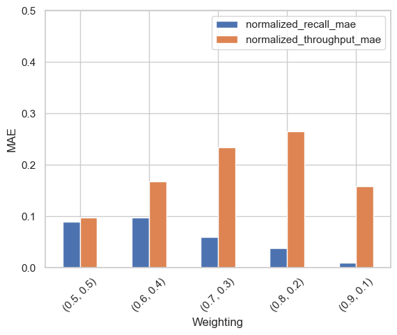
The results show that the average MAEs for normalized recall are below 0.1. For context, if dataset recall values range from 0.5 to 0.95, an MAE of 0.1 translates to a raw recall difference of only 0.045. This suggests that the predicted configurations closely match the ground truth configurations, particularly for high-recall weightings.
The MAEs for throughput are larger, likely because throughput measurements tend to be noisier than recall measurements. However, the MAEs decrease when higher weight is assigned to throughput.
Deployment evaluation
For this evaluation, we applied our method to the 15 training datasets and tested the resulting configurations on 3 datasets using the Cohere-embed-english-v3 embedding model. Our goal was to ensure that the learned configurations align with the Pareto front, representing different trade-offs between recall and throughput.
The following plot depicts the recall and throughput for the learned configurations in different colors, with other configurations displayed in gray.
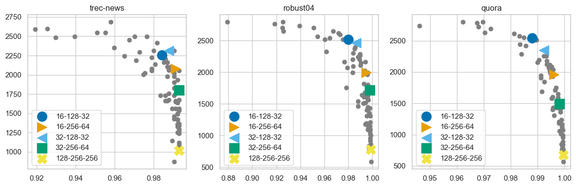
The results show that the five selected configurations effectively cover the high-recall and high-throughput regions. Because we did not assign high weights to throughput, the learned configurations do not extend into the low-recall, high-throughput area.
How to apply the configurations in OpenSearch
To try these configurations, first create an index. You must specify the index build parameters when creating the index because the parameters are not dynamic:
curl -X PUT "localhost:9200/test-index" -H 'Content-Type: application/json' -d'
{
  "settings" : {
    "knn": true
  },
  "mappings": {
    "properties": {
      "my_vector": {
        "type": "knn_vector",
        "dimension": 4,
        "space_type": "l2",
        "method": {
          "name": "hnsw",
          "parameters": {
            "m": 16,
            "ef_construction": 256
          }
        }
      }
    }
  }
}
'
Next, ingest your data:
curl -X PUT "localhost:9200/_bulk" -H 'Content-Type: application/json' -d'
{ "index": { "_index": "test-index" } }
{ "my_vector": [1.5, 5.5, 4.5, 6.4]}
{ "index": { "_index": "test-index" } }
{ "my_vector": [2.5, 3.5, 5.6, 6.7]}
{ "index": { "_index": "test-index" } }
{ "my_vector": [4.5, 5.5, 6.7, 3.7]}
{ "index": { "_index": "test-index" } }
{ "my_vector": [1.5, 5.5, 4.5, 6.4]}
'
Lastly, run a search:
curl -X GET "localhost:9200/test-index/_search?pretty&_source_excludes=my_vector" -H 'Content-Type: application/json' -d'
{
  "size": 100,
  "query": {
    "knn": {
      "my_vector": {
        "vector": [0, 0, 0, 0],
        "k": 100,
        "method_parameters": {
          "ef_search": 128
        }
      }
    }
  }
}
'
Because ef_search is a search-time parameter, it can be dynamically configured for each search request.
End-to-end example using the Python client
The following is an end-to-end example using the Python client with the boto3 and opensearch-py packages.
Load necessary modules
from typing import Tuple, List
import sys
import time
import logging
import random
import hashlib
import json

import h5py
import numpy as np
import pandas as pd
from tqdm import tqdm
import boto3

from opensearchpy import OpenSearch, RequestsHttpConnection, helpers
from opensearchpy.exceptions import RequestError, NotFoundError, TransportError
from opensearchpy.helpers.errors import BulkIndexError
from requests_aws4auth import AWS4Auth
Modify the data loading function to load your own data
The following function assumes an hdf5 file with the keys "documents", "queries", and "ground_truth":
def load_data(local_file_path: str) -> Tuple[np.ndarray, np.ndarray, np.ndarray]:
    """
    Load vector datasets from local_file_path

    Args:
        local_file_path (str): Path to the local file storing .

    Returns:
        Tuple[np.ndarray, np.ndarray, np.ndarray]:
        A tuple containing:
          - documents (np.ndarray): A set of vectors (n, m) to search against.
          - querys (np.ndarray): A set of query (q, m) vectors to test an ANN algorithm.
          - neighbors (np.ndarray): An array (q, k) that contains groundtruth top k neighbors for each query.
    """
    hdf5_file = h5py.File(local_file_path, "r")
    vectors = hdf5_file["documents"]
    query_vectors = hdf5_file["queries"]
    neighbors = hdf5_file["ground_truth"]
    return vectors, query_vectors, neighbors
Load all the util functions
logger = logging.getLogger(__name__)


def get_client(host: str, region: str, profile: str) -> OpenSearch:
    """Get an OpenSearch client using the given host and AWS region.
    It assumes AWS crediential has been configured.

    Args:
        host (str): OpenSearch domain endpoint.
        region (str): An AWS region, e.g. us-west-2

    Returns:
        OpenSearch: An OpenSearch client.
    """
    credentials = boto3.Session(profile_name=profile, region_name=region).get_credentials()

    awsauth = AWS4Auth(
        credentials.access_key,
        credentials.secret_key,
        region,
        "es",
        session_token=credentials.token,
    )

    client = OpenSearch(
        hosts=[{"host": host, "port": 443}],
        http_auth=awsauth,
        use_ssl=True,
        verify_certs=True,
        connection_class=RequestsHttpConnection,
        timeout=60 * 60 * 5,
        search_timeout=60 * 60 * 5,
    )
    return client


def create_index_body(config, engine):
    return {
        "settings": {
            "index": {"knn": True, "knn.algo_param.ef_search": config["efSearch"]},
            "number_of_shards": 1,
            "number_of_replicas": 0,
        },
        "mappings": {
            "_source": {"excludes": ["vector"], "recovery_source_excludes": ["vector"]},
            "properties": {
                "vector": {
                    "type": "knn_vector",
                    "dimension": config["dim"],
                    "method": {
                        "name": "hnsw",
                        "space_type": config["space"],
                        "engine": engine,
                        "parameters": {
                            "ef_construction": config["efConstruction"],
                            "m": config["M"],
                        },
                    },
                }
            },
        },
    }


def get_index_name(config: dict) -> str:
    """Hash the config dict to get a unique index name

    Args:
        config (dict): An HNSW configuration to evaluate.

    Returns:
        str: A unique index name using hashing.
    """
    dict_str = "_".join(map(str, config.values()))
    hash_obj = hashlib.md5(dict_str.encode())
    index_name = hash_obj.hexdigest()
    return index_name


def random_delay(lower_time_limit: float = 1.0, upper_time_limit: float = 2.0) -> float:
    return min(lower_time_limit + random.random() * upper_time_limit, upper_time_limit)


def bulk_index_vectors(
    client: OpenSearch,
    index: str,
    vectors: List[np.ndarray],
    source_name: str,
    batch_size=1000,
):
    """Bulk ingesting vectors with batch_size into index with name index_name

    Args:
        client (OpenSearch): An OpenSearch client
        index (str): Index to ingest vectors.
        vectors (List[np.ndarray]): List of vectors to be ingested.
        source_name (str): Name to be used in the `_source` field.
        batch_size (int, optional): Defaults to 1000.
    """
    actions = []
    for i, vector in enumerate(
        tqdm(vectors, desc="Indexing vectors", total=len(vectors), file=sys.stdout)
    ):
        # Create an index request for each vector
        action = {
            "_index": index,
            "_id": i,  # Unique ID for each vector
            "_source": {source_name: vector.tolist()},  # Convert NumPy array to list
        }
        actions.append(action)

        # When the batch size is reached, send the bulk request
        if len(actions) == batch_size:
            helpers.bulk(client, actions)
            actions = []  # Clear actions for the next batch

    # Index any remaining documents that didn't fill the batch size
    if actions:
        helpers.bulk(client, actions)


def delete_one_index(client: OpenSearch, index: str, max_retry: int = 5):
    try:
        client.indices.clear_cache(
            index=index, fielddata=True, query=True, request=True
        )
    except NotFoundError:
        pass

    success = False
    count = 0
    while not success and count < max_retry:
        try:
            client.indices.delete(index=index)
            success = True
        except NotFoundError:
            logger.error(f"{index} not found, SKIP.")
            success = True
        except RequestError as e:
            delay = random_delay()
            logger.error(f"{index} delete failed {e}, wait {delay} seconds.")
            time.sleep(delay)
        count += 1


def get_graph_memory(client: OpenSearch) -> float:
    resp = client.transport.perform_request(
        method="GET", url=f"/_plugins/_knn/stats?pretty"
    )
    return sum([stat["graph_memory_usage"] for node_id, stat in resp["nodes"].items()])


def knn_bulk_search(client, config, index_name, query_vectors, k):
    # Prepare the msearch request body
    msearch_body = ""
    for query_vector in query_vectors:
        search_header = '{"index": "' + index_name + '"}\n'
        search_body = {
            "size": k,
            "query": {
                "knn": {
                    "vector": {
                        "vector": query_vector.tolist(),  # Convert NumPy array to list
                        "k": k,
                    }
                }
            },
            "_source": False,
        }

        # Append header and body for each query to the msearch body
        msearch_body += search_header + json.dumps(search_body) + "\n"

    # Send the msearch request
    response = client.msearch(body=msearch_body)
    return response


def pad_list(input_list, n):
    """
    Pads the input list with -1 on the right if its length is less than n.

    :param input_list: List of integers to pad
    :param n: The desired length of the list
    :return: The padded list
    """
    if len(input_list) < n:
        input_list += [-1] * (n - len(input_list))
    return input_list


def batch_knn_search(client, config, index_name, query_vectors, batch_size, k):
    pred_inds = []
    took_time = 0.0
    for i in tqdm(
        range(0, len(query_vectors), batch_size), desc="Search vectors", file=sys.stdout
    ):
        batch = query_vectors[i : i + batch_size]
        results = knn_bulk_search(client, config, index_name, batch, k)
        # Process results for each batch
        for j, result in enumerate(results["responses"]):
            ids = [hit["_id"] for hit in result["hits"]["hits"]]
            if len(ids) < k:
                logger.error(f"{config} batch {i} search needs padding")
                ids = pad_list(ids, k)
            pred_inds.append(ids)
        took_time += results["took"]
    return pred_inds, took_time * 0.001 # convert took_time from ms to s.


def compute_recall(labels: np.ndarray, pred_labels: np.ndarray):
    assert labels.shape[0] == pred_labels.shape[0], (
        labels.shape,
        pred_labels.shape,
    )
    assert labels.shape[1] == pred_labels.shape[1], (
        labels.shape,
        pred_labels.shape,
    )
    labels = labels.astype(int)
    pred_labels = pred_labels.astype(int)
    k = labels.shape[1]
    correct = 0
    for pred, truth in zip(pred_labels, labels):
        top_k_pred, truth_k = pred[:k], truth[:k]
        for p in top_k_pred:
            for y in truth_k:
                if p == y:
                    correct += 1
    return float(correct) / (k * labels.shape[0])


def ingest_vectors(
    config: dict,
    engine: str,
    client: OpenSearch,
    index_name: str,
    vectors: List[np.ndarray],
):
    index_body = create_index_body(config, engine)

    success = False
    max_try = 0
    while not success and max_try < 5:
        try:
            client.indices.create(index=index_name, body=index_body)
            logger.info(f"{index_name}: Ingesting vectors")
            bulk_index_vectors(client, index_name, vectors, "vector")
            success = True
        except BulkIndexError as e:
            delay = random_delay()
            delete_one_index(client, index_name)
            max_try += 1
            time.sleep(random_delay())
            logger.error(
                f"{index_name}: BulkIndexError, retrying after {delay} seconds\n{e}"
            )
        except RequestError as e:
            if e.error == "resource_already_exists_exception":
                delay = random_delay()
                logger.error(f"{e}, delete and retry after {delay} seconds")
                delete_one_index(client, index_name)
                time.sleep(random_delay())
                max_try += 1
            else:
                raise


def query_index(config, index_name, client, query_vectors, k) -> list[np.ndarray]:
    success = False
    batch_size = 100  # large batch size may lead to query time out
    max_try = 0
    while not success and max_try < 5:
        try:
            pred_inds, search_time = batch_knn_search(
                client, config, index_name, query_vectors, batch_size=batch_size, k=k
            )
            success = True
            return pred_inds, search_time
        except TransportError as e:
            delay = random_delay()
            logger.error(
                f"{index_name}: Query failed, retrying after {delay} seconds {e}"
            )
            time.sleep(delay)
            max_try += 1
    raise Exception(f"{index_name}: Query failed after {max_try} retries")


def eval_config(
    config: dict, local_file_path: str, host: str, region: str, aws_profile: str, engine: str, k=10
):

    vectors, query_vectors, neighbors = load_data(local_file_path)
    client = get_client(host, region, aws_profile)  # creat new one to avoid credential expiring
    index_name = get_index_name(config)

    ingest_vectors(config, engine, client, index_name, vectors)

    # prepare for searching
    client.transport.perform_request(method="POST", url=f"/{index_name}/_refresh")
    client.transport.perform_request(
        method="GET", url=f"/_plugins/_knn/warmup/{index_name}?pretty"
    )
    stats = client.indices.stats(index=index_name, metric="store")
    index_size_in_bytes = stats["indices"][index_name]["total"]["store"][
        "size_in_bytes"
    ]
    graph_mem_in_kb = get_graph_memory(client)

    time.sleep(random_delay(lower_time_limit=5, upper_time_limit=10))

    logger.info(f"{index_name}: Query indexes")
    pred_inds, search_time = query_index(config, index_name, client, query_vectors, k)

    groundtruth_topk_neighbors = [v[:k] for v in neighbors]
    recall = compute_recall(np.array(groundtruth_topk_neighbors), np.array(pred_inds))
    logger.info(f"{index_name}: Recall {recall}")

    config.update(
        {
            f"recall@{k}": recall,
            "search_time": search_time,
            "search_throughput": len(query_vectors) / search_time,
            "index_size_in_bytes": index_size_in_bytes,
            "graph_mem_in_kb": graph_mem_in_kb,
        }
    )

    # clean up
    delete_one_index(client, index_name)
    logger.info(f"Clean up done, finishing evaluation.")
    return config
Define the variables for your experiments
Define the following variables for your experiments:
- OpenSearch domain and engine
- AWS Region and AWS profile
- Local file path
- Dataset dimension
- Space to use in HNSW
host = "your_domain_endpoint_without_https://"
engine = "faiss"

region = "us-west-2"
aws_profile = "your_aws_profile"

local_file_path = "your_data_path"
dim = 384 # vector dimension
space = "l2" # space in HNSW
Evaluate different configurations
metrics = []
for i, config in enumerate([
    {'M': 16, 'efConstruction': 128, 'efSearch': 32},
    {'M': 32, 'efConstruction': 128, 'efSearch': 32},
    {'M': 16, 'efConstruction': 128, 'efSearch': 128},
    {'M': 64, 'efConstruction': 128, 'efSearch': 128},
    {'M': 128, 'efConstruction': 256, 'efSearch': 256}
]):
    config.update({"dim": dim, "space": space})
    metric = eval_config(config, local_file_path, host, region, aws_profile, engine)
    metrics.append(metric)
You will see the following output in the terminal:
Indexing vectors: 100%|██████████| 8674/8674 [00:26<00:00, 321.72it/s]
Search vectors: 100%|██████████| 15/15 [00:09<00:00,  1.55it/s]
Indexing vectors: 100%|██████████| 8674/8674 [00:34<00:00, 248.95it/s]
Search vectors: 100%|██████████| 15/15 [00:07<00:00,  1.88it/s]
Indexing vectors: 100%|██████████| 8674/8674 [00:30<00:00, 280.84it/s]
Search vectors: 100%|██████████| 15/15 [00:07<00:00,  2.09it/s]
Indexing vectors: 100%|██████████| 8674/8674 [00:27<00:00, 311.41it/s]
Search vectors: 100%|██████████| 15/15 [00:07<00:00,  2.07it/s]
Indexing vectors: 100%|██████████| 8674/8674 [00:34<00:00, 250.86it/s]
Search vectors: 100%|██████████| 15/15 [00:07<00:00,  2.03it/s]
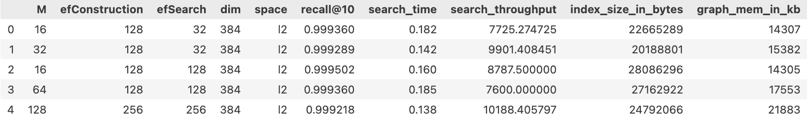
You can visualize the metrics by running the following code:
df = pd.DataFrame(metrics)
df
The following image depicts an example metric visualization.
Limitations and future work
This blog post focuses on optimizing HNSW for two key objectives: recall and throughput. However, to further adjust the size of the HNSW graph, exploring different values for ef_construction could provide additional insights.
Our method currently generates the same set of configurations across all datasets, but this approach can potentially be improved. By considering the specific characteristics of each dataset, we could create more targeted recommendations. Additionally, the current set of configurations is based on 15 datasets. Incorporating a broader range of datasets into the training process would enhance the generalization of the learned configurations.
Looking ahead, expanding the scope to include recommendations for quantization methods alongside HNSW could further reduce index size and improve throughput.
References
- Malkov, Yu A., and Dmitry A. Yashunin. “Efficient and robust approximate nearest neighbor search using hierarchical navigable small world graphs.” IEEE transactions on pattern analysis and machine intelligence 42.4 (2018): 824-836.
- Xu, Lin, Holger Hoos, and Kevin Leyton-Brown. “Hydra: Automatically configuring algorithms for portfolio-based selection.” Proceedings of the AAAI Conference on Artificial Intelligence. Vol. 24. No. 1. 2010.
- Winkelmolen, Fela, et al. “Practical and sample efficient zero-shot hpo.” arXiv preprint arXiv:2007.13382 (2020).
- Salinas, David, and Nick Erickson. “TabRepo: A Large Scale Repository of Tabular Model Evaluations and its AutoML Applications.” arXiv preprint arXiv:2311.02971 (2023).
- Feurer, Matthias, and Frank Hutter. Hyperparameter optimization. Springer International Publishing, 2019.
- Shahriari, Bobak, et al. “Taking the human out of the loop: A review of Bayesian optimization.” Proceedings of the IEEE 104.1 (2015): 148-175.